The Context Layer Is Emerging — Here’s an Open Schema for It
The data industry is converging on a single idea: AI agents need structured context beyond raw schemas. And the tooling is being built right now.
dbt Labs published a four-part blog series in late 2025 titled “Bringing Structured Context to AI with dbt.” Databricks added semantic metadata to metric views — synonyms, display names, format specs — explicitly designed for their Genie AI assistant. Google shipped a Looker MCP server claiming it “reduces data errors in gen AI natural language queries by as much as two thirds.” Cube.js rebranded as an “agentic analytics platform.” ThoughtSpot’s Spotter uses “Models” with synonyms, keywords, and join paths. Atlan launched “context graphs” positioned as “knowledge graphs enhanced with operational metadata.”
All of them are solving the same foundational problem: how to find and compute metrics. Definitions, lineage, ownership, join paths, synonyms, access controls. The semantic layer tells the AI what revenue means and how to calculate it. This is necessary and real progress.
The next frontier is encoding what happens after computation: What should revenue look like? When it drops, where do you look first? What else moves when revenue moves? What do you do about it? Is there an SLA?
That operational knowledge — the institutional context that distinguishes a senior analyst’s investigation from a junior analyst’s flat list of “things to check” — lives in wiki pages, Slack threads, incident reports, onboarding notes, and people’s heads. It decays fast. It’s the most valuable and most fragile knowledge an organization has about its metrics.
Everyone agrees the gap exists. Nobody published a schema for filling it.
This article describes one: a 36-field, 5-layer structure that encodes operational metric knowledge directly in dbt MetricFlow YAML — co-located with the metric definition, version-controlled in git, queryable by any tool that reads YAML. We tested it empirically across three Claude models and six context conditions. The result: Haiku + structured meta context matches Opus + scattered documentation. The cheapest model with the right context achieves the quality of the most expensive model with the wrong context.
Everyone else is building context for finding and computing metrics. This schema builds context for understanding and investigating them.
Five Layers, Five Failure Modes
The five layers weren’t designed from theory. They were discovered empirically and then explained with theory.
We took a single metric (order_success_rate) and wrote six versions of its YAML, each adding one layer of business context:
| Version | What’s added | What changes |
|---|---|---|
| V0 | Bare metric definition | LLM can describe the computation but can’t assess severity, suggest causes, or recommend actions |
| V1 | + Context (purpose, owner) | Interpretation improves — but still can’t tell good from bad |
| V2 | + Expectations (ranges, thresholds, seasonality) | Step-change. “87% is below warning threshold” — but investigation is generic |
| V3 | + Investigation (causal dimensions, decision tree) | Structured investigation: “check fulfillment_channel first because…” |
| V4 | + Relationships (correlations, external events) | Connects cross-metric patterns — but confidently fabricates SLAs |
| V5 | + Decisions (action protocols, business rules) | False confidence eliminated. Correctly states “no SLA documented” |
Three findings stood out:
Non-linearity. V1→V2 and V4→V5 produced step-changes. Other transitions were gradual. The layers aren’t arbitrary — each closes a distinct failure mode.
The dangerous middle. V2-V4 (expectations without business rules) was more dangerous than V0 (no context at all). An LLM with calibration data but no decision constraints gives confidently wrong answers about SLAs. Partial context creates false confidence.
Order matters. You can’t skip Layer 2 and still benefit from Layer 3 — without calibration, investigation paths have no trigger. And you can’t have Layer 2 without Layer 5 — expectations without decision constraints are dangerous.
Each layer maps to a specific reasoning failure:
| Layer | The question | The failure without it |
|---|---|---|
| Context | “Who cares and why?” | Interpretation failure — computes amounts but doesn’t apply the business formula |
| Expectations | “What does good look like?” | Calibration failure — can’t tell if 87% is normal or catastrophic |
| Investigation | “Where do I look first?” | Framing failure — flat list instead of a prioritized decision tree |
| Relationships | “What else moves?” | Reasoning failure — analyzes the metric in isolation |
| Decisions | “What do I do?” | Action failure — either “further analysis recommended” (useless) or invented SLAs (dangerous) |
Structured Meta Outperformed Scattered Docs Across All Three Models
Most documentation organizes knowledge by topic — “About this metric,” “Troubleshooting,” “Related metrics.” This works for sequential human reading but fails for LLM retrieval. When an LLM needs to assess severity, it has to extract calibration data from a section titled “About this metric” (where thresholds might be mentioned in passing), cross-reference with “Troubleshooting” (where severity might be implied), and hope “Related metrics” mentions magnitude.
The 5-layer structure organizes by reasoning operation:
| When the LLM needs to… | It looks at exactly… | Not scattered across… |
|---|---|---|
| Interpret the number | context.purpose | wiki page, README, old email |
| Assess severity | expectations.healthy_range | footnotes, PagerDuty configs, tribal knowledge |
| Frame the investigation | investigation.causal_dimensions | post-mortems, Slack threads |
| Connect to other signals | relationships.correlates_with | architecture diagrams, incident reports |
| Recommend action | decisions.when_this_drops | SLA docs, runbooks, regulatory filings |
Each layer is a retrieval unit — all the knowledge needed for one type of reasoning, in one place, with no filler. The performance difference isn’t about content — it’s about retrieval architecture.
We tested this directly.
Scattered Docs vs. Co-located Meta
We created 13 fictitious documents for a spend analytics metric (merchant_auth_decline_rate): 7 scattered docs, 3 distractor docs, a ground truth answer key, and two schema variants (bare and meta-enriched). The key trap: the operational runbook says the critical threshold is >15%, but a buried email thread documents a change to 18%, confirmed in a quarterly review. The meta block has the single canonical value (18%).
Five questions, one per failure type. Scored on 5 dimensions against the ground truth. Six conditions: bare metric definition, structured meta, clean docs (2 relevant documents), full docs (all 7), and adversarial (10+ including distractors).
The results changed the story
| Condition | Haiku | Sonnet | Opus |
|---|---|---|---|
| Bare definition | 2.3 | 3.0 | 3.1 |
| Structured meta | 4.7 | 4.9 | 4.9 |
| Clean docs (2 docs) | 3.8 | 4.2 | 4.5 |
| Full docs (7 docs) | 4.0 | 4.4 | 4.5 |
| Adversarial docs (10+) | 4.1 | 4.5 | 4.6 |
Three things surprised us:
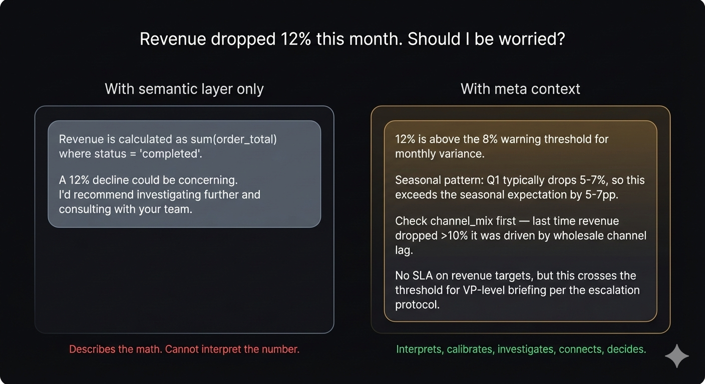
The calibration gap is the biggest single step-change. The bare definition literally says “it is not possible to say definitively whether 12% is concerning.” With structured meta, the answer is immediate: “12% is at the warning threshold” with exact numbers, seasonality context, and segmentation advice. This is the difference between a tool that describes numbers and one that interprets them.
More docs ≠ better answers. Full docs (7 docs, ~4,700 words) scored the same as clean docs (2 docs, ~1,800 words). The additional documents provided richer investigation examples but introduced the threshold contradiction that hurt decision quality. Adding more context made the system work harder without making it work better.
Opus was too robust for the adversarial condition. Adversarial docs actually scored higher than full docs — Opus correctly ignored the distractors. This is a model capability ceiling, which makes the next finding even more important.
Haiku + Meta Context Matched Opus + Scattered Docs
Read the rightmost column:
| Condition | Haiku | Opus | Gap |
|---|---|---|---|
| Bare definition | 2.3 | 3.1 | 0.8 |
| Structured meta | 4.7 | 4.9 | 0.2 |
| Full docs | 4.0 | 4.5 | 0.5 |
Without context, there’s a 0.8-point gap between Haiku and Opus — model capability drives performance. With meta context, the gap compresses to 0.2. All three models converge near 4.8+.
The meta block is doing the reasoning work that separates model tiers. Threshold reconciliation, investigation path prioritization, relationship typing, SLA verification — these are the tasks Opus handles well and Haiku handles poorly when working from raw documents. The meta block moves all of those tasks to authoring time, where they’re done once by a capable model, and the results are served to any model at query time.
The headline finding: Haiku + meta context (4.7) matches or exceeds Opus + scattered docs (4.6). The cheapest model with structured context achieves the quality level of the most expensive model with unstructured context.
The per-question breakdown reveals where:
| Question | Haiku (bare) | Haiku (meta) | What meta provides |
|---|---|---|---|
| Calibration | 2.0 | 4.8 | Exact thresholds — Haiku can’t reconcile contradictory docs |
| Investigation | 2.2 | 4.8 | Prioritized path — Haiku follows encoded priority but can’t derive it |
| Decision | 2.0 | 4.8 | Explicit no-SLA — Haiku with docs still uses the old 15% threshold |
Calibration and decision show the largest gaps — exactly where threshold precision and SLA knowledge matter, and exactly where Haiku struggles with scattered docs. Haiku can’t do source reconciliation at query time. Opus can. Meta eliminates the need.
You Already Have the Knowledge — It Just Needs Extracting
Before testing weaker models, we asked a different question: does populating the meta block require someone who already knows all the answers?
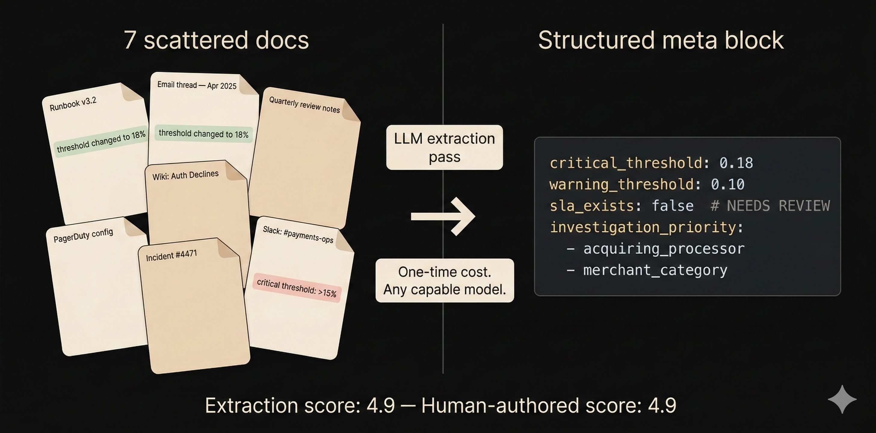
We pointed an extraction prompt at the same 7 scattered docs and let it synthesize the meta block. Results: 33 of 36 fields populated, 13/13 Core fields at 100%. The extraction correctly reconciled the threshold contradiction (resolving to 18% with a # NEEDS REVIEW: Runbook still shows 15% annotation), synthesized a branching investigation path from three different sources, and made a positive assertion of SLA absence rather than silence.
The extracted meta scored 4.9 — matching the version we’d authored with full knowledge of the ground truth. In one case the extraction was more accurate: our version had the wrong warning threshold (0.12 vs. the correct 0.10 from the email thread). The mechanical extraction was more faithful to the sources than we were.
The implication: the knowledge to populate the schema already exists in your organization’s docs, runbooks, and Slack threads. An LLM extraction pass structures it — without the errors that come from trying to remember everything yourself.
Encode Once, Query Forever
The multi-model finding changes the cost calculus entirely.
Without meta context, every question pays the full reasoning tax. “Is 12% concerning?” requires finding the relevant docs, extracting threshold values, noticing the contradiction, reconciling it, assessing severity, and composing an answer. This chain requires a capable model — Opus or equivalent — because weaker models fail at the reconciliation step.
With meta context, that reasoning was done once at extraction time. “Is 12% concerning?” resolves to: read warning_threshold: 0.10, read critical_threshold: 0.18, compare, report. Haiku can do this.
| Approach | Per-query cost | Quality |
|---|---|---|
| Haiku + no context | $ | 2.3 |
| Haiku + meta | $ | 4.7 |
| Sonnet + scattered docs | $$$ | 4.4 |
| Opus + scattered docs | $$$$$ | 4.6 |
An organization with 500 analysts asking questions about 200 metrics isn’t paying for 100,000 document-reconciliation tasks at Opus prices. It’s paying for 200 extraction tasks once, then serving answers at Haiku prices — indefinitely.
Meta context is compiled knowledge. You pay the compile cost once, then every read is cheap. And the extraction itself gets cheaper over time — today’s Opus becomes next year’s Sonnet at last year’s Haiku prices, but the meta block it authored is model-agnostic YAML.
Every AI Answer Becomes Auditable
The cost argument is compelling but insufficient. Meta context has a property that scattered documentation structurally cannot have: temporal queryability.
On March 1st, an agent says “15% is at the critical threshold — escalate immediately.” On March 10th, someone asks: was the agent right to escalate? With scattered documentation, this question is unanswerable. Which version of which wiki page was in the context window? Had the email thread about the threshold change been indexed yet?
With meta context in version-controlled YAML:
git show <commit-at-march-1>:models/mart_spend/schema.ymlOne command reconstructs exactly what the meta block said. What the critical threshold was. What the investigation path recommended. Whether the no-SLA assertion was present. The meta block is the agent’s epistemic state made explicit — frozen in git, queryable at any point in time.
Justin Johnson, discussing what knowledge graphs must be able to do, posed a test:
“Can your system tell me what a specific agent knew at 2:14 PM last Tuesday when it made a specific decision?”
With scattered documentation — no. With meta context in version-controlled YAML — yes.
This is what makes meta context more than an optimization. It’s not just faster, cheaper, or more accurate. It’s accountable.
At Portfolio Scale: The Meta Block Becomes a Graph
Everything so far describes what meta context does for a single metric. The picture changes when you have 200.
Each meta block has a primary key (the metric name it’s attached to) and foreign keys embedded in its fields: owner points to a team, correlates_with creates metric-to-metric edges, causal_dimensions links to semantic layer dimensions, affected_by connects to external events. Extract 200 meta blocks into a relational structure and you get five tables:
metrics            (metric_name PK, owner, domain, healthy_range, thresholds, ...)
metric_edges       (source_metric FK, target_metric FK, relationship_type, direction)
metric_dimensions  (metric_name FK, dimension_name FK, investigation_priority)
metric_events      (metric_name FK, event_type, magnitude, last_occurrence)
metric_escalation  (metric_name FK, role, threshold_trigger)
That’s not a documentation format. That’s a knowledge graph with typed edges — and graphs are queryable in ways that documentation cannot be.
Blast radius. “Worldpay is reporting an outage. Which metrics are affected and who needs to know?” No wiki page answers this. But query metric_events for Worldpay, join to metric_escalation for the people, traverse correlates_with edges for second-order impacts — and you get a specific list of metrics, owners, and thresholds. Not “check everything.” A targeted response.
Shared-cause detection. Three metrics spike in the same hour. Are they connected, or is this coincidence? Check whether they share causal_dimensions. If all three list acquiring_processor as a top-priority investigation dimension, that’s a strong signal — the shared dimension suggests a shared root cause. The agent doesn’t need to guess; the graph encodes the relationship.
Coverage gaps as risk signals. “Which metrics have expectations (thresholds, ranges) but no decision rules?” These are the false-confidence risks we identified in the ablation — metrics where the agent can assess severity but might fabricate SLA obligations. A portfolio scan surfaces them systematically instead of waiting for an incident.
Ownership continuity. Marcus is on vacation. Which metrics are in his escalation path? Are any currently above warning threshold? Who’s the backup? This is the kind of question that, today, gets answered by Slack DMs to people who might not answer.
Graph integrity as a quality signal. Metric A says it correlates with Metric B, but B’s meta block doesn’t mention A. Either the relationship is asymmetric (document why) or one block is incomplete. A linter catches this automatically — referential integrity for business knowledge.
The graph property compounds the cost advantage from earlier. Without the graph, an agent answering a multi-metric question (“three metrics spiked — are they connected?”) must search for and reconcile documentation across 3 × N documents. With the graph, it reads 3 meta blocks and traverses their edges. Single-metric queries scale linearly with document count; multi-metric queries scale quadratically. The meta graph makes multi-metric reasoning tractable at Haiku prices.
And the graph itself represents organizational knowledge that no document contains. No wiki page says “here are all the metrics affected by a Worldpay outage, ranked by severity.” That knowledge lives in the heads of senior analysts. The meta schema makes it explicit, structured, and queryable — by any model, at any time, at any point in git history.
Endnotes
A. Example Exchanges by Question Type
Each of the five layers serves a progressively deeper analytical question. Here are worked examples using a disbursement success rate metric.
Descriptive — “What is this metric?”
Without Layer 1: “It’s a ratio of completed_count to transaction_count.”
With Layer 1: “It measures the share of all disbursement transactions (OCT + RTP combined) that complete successfully. Denominator is total initiated; numerator is completed (not reversed). It’s the headline health metric for the disbursements pipeline.”
Evaluative — “Is this number good or bad?”
Without Layer 2: “A drop to 88% could be concerning. I’d recommend investigating further.”
With Layer 2: “88% is below the 92% warning threshold but above the 85% critical threshold. The healthy range is 94-99%. Note: Dayforce rail historically ranges 76-94%, so if the system-wide drop is driven entirely by Dayforce, this may be within normal operating range for that program.”
Diagnostic — “Why did this happen?”
Without Layer 3: “Consider checking: calendar_date trends, program_code distribution, processor status, transaction amounts, and status codes.”
With Layer 3: “First: check program_code breakdown — is this one rail or all? Each BaaS program has different success profiles; Dayforce alone swung 17pp in Jul 2025. IF system-wide: check processor status. IF single rail with Dayforce: check bank connectivity (historically volatile). IF Flex specifically: unusual — check data quality.”
Systemic — “What else is affected?”
Without Layer 4: “I can only analyze disbursement_success_rate. You might want to check other metrics.”
With Layer 4: “disbursement_success_rate is inversely related to both decline_rate and failure_rate (success + decline + failure ≈ 1.0). Check: is the drop showing up as increased declines (pre-execution) or failures (post-execution)? These have different root causes.”
Decisional — “What should I do?”
Without Layer 5: “88% appears to be below normal levels. You may want to escalate to your operations team.”
With Layer 5: “88% is below the 92% warning threshold. Action: check program_code breakdown. Note: No formal SLA on disbursement success rate is currently documented — treat thresholds as analytical guidelines, not contractual obligations.”
C. Placement Rules: Not Every Field on Every Metric
If you have 30 metrics on a model, you don’t need 30 full meta blocks. dbt’s meta: property exists at both the semantic model level and the metric level. Model-level fields are shared; metric-level fields override where they diverge.
The rule: if changing a field’s value for one metric but not another would be wrong, it belongs at the metric level. If it would be redundant, it belongs at the model level.
In practice: Context (~70% shareable) lives mostly at the model level — owner, data source, grain. Expectations (~20% shareable) and Decisions (~20%) live at the metric level — ranges, thresholds, and action protocols diverge per metric. For a model with 22 metrics, this means ~8 fields per metric, not 36.
D. Related Work
We haven’t found a published structure that maps specific LLM failure types to specific categories of business knowledge in a layered schema. But several practitioners informed the design:
- Jessica Talisman argued that meaning has architecture — layers of increasing semantic richness. Her principle that meaning is layered, not flat is foundational. Her process knowledge work argues that procedural knowledge (how experts investigate, what decisions they make) is the most valuable and fastest-decaying — exactly what Layers 3 and 5 encode.
- Brian Jin identified four mechanisms of context decay: speed of decision-making, wrong storage medium, personnel rotation, temporal drift. His argument that investigation logic is the highest-decay organizational knowledge is why Layer 3 exists as its own layer.
- Chris Gambill proposed a 3-layer metadata anatomy (Technical, Process, Business). Our Layers 3-5 extend beyond his Business metadata into investigation, relationships, and decisions.
- Shane Butler proposed a layered validation system where logical coherence requires baselines — directly motivating Layer 2.
E. Limitations
This evaluation is a controlled simulation, not a production deployment.
Sample size: N=1 per condition per model. The direction is consistent, but specific score differences (4.7 vs 4.6) are within scoring noise.
Simulated documents: The threshold contradiction was designed. Real-world documentation may have more contradictions (making the case for meta stronger) or fewer.
Scoring methodology: Answers scored by the researchers who designed the study. A blinded LLM-as-judge scorer is a planned extension.
Single domain, single provider. One fictitious metric, three Anthropic models. Cross-domain and cross-provider testing are planned.
Maintenance cost. The economics section compares query-time costs but doesn’t fully account for keeping meta blocks current. A production pilot would quantify this.